Elementarization and Modularization
-
Two didactical aims being realized
by using Computeralgebra Systems
by Klaus Aspetsberger
Paedagogische Akademie des Bundes in Oberoesterreich
Kaplanhofstrasse 40, A-4020 Linz, Austria, Europe
It is obvious to use computeralgebra systems (CAS) as a calculating aid for dedicating tasks as solving equations, computing limits and derivatives, etc. to the computer. However, CAS can also be used for introducing new mathematical concepts, e.g., solving problems for changing rates by computing sequences of differences is much more elementary than using derivatives. So CAS are a valuable help for introducing and elementarizing new mathematical concepts. Using CAS students have the possibility to define functions in a very similar way as they were used in regular maths lessons or textbooks. So CAS are an important instrument for modularizing maths teaching.
1. Introduction
We report about mathematics courses in a class with 12 girls and 3 boys
at the age of 16 in the years from 1995 to 1998 at the Stiftsgymnasium
Wilhering, which is a private High School near Linz in Austria. The emphasis
of the school and the interests of the students are in the study of languages
and arts. Because the students are not intrinsically motivated in mathematics,
it is our aim, to make new mathematical concepts easy to understand for
them by treating and computing them in a very elementary way. All students
use a TI-92, which is a pocket calculator for symbolic and numerical manipulations
and for graphical visualizations. The students use the TI-92 during maths
classes, at home for doing exercises and during maths tests.
2. Elementarization
In the following examples we demonstrate how one can use a computeralgebra
system (CAS) for introducing new mathematical contents. The experiences
we will describe are made with the TI-92, however the didactical concepts
could be transferred to other CAS products.
Exponential functions
In traditional maths courses exponential functions are introduced as functions
of the type a*. Most of the time is spent for proving and training transformation
rules or for solving exponential equations. There is not much time for
the students to learn about the meaning of a and in which situations
exponential functions are necessary for modelling a process and how exponential
functions differ from other types of functions.
Using CAS we can concentrate on the modelling process. Dedious and complicated
computations can be dedicated to the CAS. Furthermore the modelling process
is supported by the possibility of defining sequences recursively. Consider
the following example of a population of 1000 individuals with a procedual
growing rate of 5 % per year. The growing process of this population can
be described recursively as follows: Pn=Pn-1+ Pn-1*0.05
with P0=1000 . In this recursive description the amount of
absolute growth Pn-1*0.05 can be easily inspected. It depends
on the number of individuals in the past year. This is a characteristic
difference of exponential growth to other growing processes, e.g. linear
growth where the amount of absolute growth is constant.
In contrast to the closed form Pn=1000*1.05n of
exponential processes the recursive definitions only require addition/subtraction
and multiplication/division for modelling. This is very helpful for the
students, because they are familiar with these elmentary operations. So
it is easier for them to understand the models or to do the modelling
process by themselves ([ Aspetsberger, Fuchs 1996] , [ Schneider
1998] , [ Wurnig 1996] ).
Differentialquotient
Using CAS we can stepwise introduce the definition of differential quotients by generating and analyzing sequences of difference quotients. For solving problems we can use the definition above, because the computation of the limit is dedicated to the CAS. So the process of changing rates is always visual for the students.
In the following we present an example for a stepwise introduction of differential quotients [ Aspetsberger 1997] treating the problem of velocity [ Finney, Thomas, Demana, Waits 1994] ).
A rock is thrown straight up with a launch velocity of 64 m/sec. It reaches a height of s(t)=64t- 5t² m after t seconds.
- Compute the average velocity of the rock within the first two seconds.
- Compute the instantaneous velocity after 2 seconds.
After
entering the definition for the height s(x) of the rock, where
x denotes the time past since the shooting of the rock, the students
can easily plot the graph of the function for a first inspection. For
computing the average velocity of the rock for the first two seconds
we enter the expression ![]() (see
figure 1).
(see
figure 1).
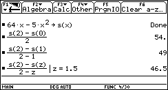
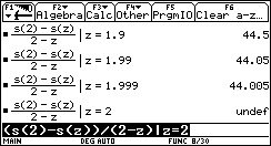
For computing the limit of
| c. How high does the rock go and when does it reach its higest point? |
On its highest point the velocity of the rock is zero. However we do not
know, when this will happen. So we can compute the instantaneous velocity
of the rock at various times for instance t = 1, 2, 4, 5 and so
on. This leads us to generalize the problem and to compute ![]() obtaining a general expression -2*(5*t-32) for the velocity of
the rock. If we store the expression to the function v(t)
we can easily compute the velocity at any time via a function call. This
is a very natural introduction of the concept of derivatives, because
students understand now why generalization is necessary. By solving the
equation v(t) = 0 we find out when the rock reaches its
highest point. The maximal height can be computed by the function call
s(32/5).
obtaining a general expression -2*(5*t-32) for the velocity of
the rock. If we store the expression to the function v(t)
we can easily compute the velocity at any time via a function call. This
is a very natural introduction of the concept of derivatives, because
students understand now why generalization is necessary. By solving the
equation v(t) = 0 we find out when the rock reaches its
highest point. The maximal height can be computed by the function call
s(32/5).
Now the students can solve many problems from various application fields
using the definition of the differential quotient directly, dedicating
the computation of the limit to the CAS.
Integrals
In traditional maths courses many teachers choose the concept of antiderivatives
for introducing integrals. They do not use upper and lower rectangular
sums because the computation of sums are rather time consuming and the
determination of closed forms for sums are quite difficult. However the
concept of antiderivatives is not as illustrative as the concept of Riemann
sums and the students do not see why antiderivatives are suitable to solve
a certain problem. Most of time is spent for computing and training of
special integration techniques by hand instead of concentrating on the
modelling process for various application areas. So they restrict to problems
of computing the area between curves.
Using CAS we can solve problems using upper and lower rectangular sums
quite conveniently dedicating the dedious work and determining closed
forms to the computer. During the whole process the students have only
to concentrate on modelling. An introduction of integrals via Riemann
sums on the TI-92 is described in [ Aspetsberger 1998] . Starting
with simple sums of products the students are guided to the general description
of Riemann sums and finally to integral functions.
Solving integral problems via Riemann sums with CAS make the process of
constructing sums always visible for the students. This is a good training
for modelling integrands. Sums are much more elementary than antiderivatives.
So the students have a chance to understand what happens. The students
do not have to take care of how to compute difficult integrals, so they
can solve various problems from different application areas. The computation
of the area between graphs is only one special application of the integral
concept.
By
the use of a CAS/TI-92 it is possible to solve problems in a very elementary
way and new mathematical concepts can be introduced stepwise. It is easier
for students to understand the meaning of a new concept when it is introduced
elementary.
However introducing new concepts very elementary may lead to incorrect
generalizations. An exact formularion and a theoretical treatment of the
new concepts are still not superflous. One can start with elementary problems
from well known application areas for introducing new maths concepts and
continue with a phase of exactification.
For solving problems the students use various methods in different representation
modes. Experimental attempts are preferred to algebraic methods.
3. Modularization
Using CAS students have the possibility to define functions in a very
similar way as they were used in regular maths lessons or textbooks. During
problem solving the students can subdivide a problem in a several number
of subproblems that can be solved independently. For solving the subproblems
the students can use functions which are already implemented in the CAS
or define new functions by themselves, generating a set of modules to
be used in standard situations. So the use of functions is an important
aid for structured problem solving. Again the use of modules by hand is
quite laborious and the advantages of functions can be seen hardly by
students. So CAS are an important instrument for modularizing maths teaching.
Using functions in maths lessons we have to distinguish between functions
which have been defined by the students themselves and functions which
are already implemented on the CAS or have been generated by the teacher
([ Aspetsberger 1996] , [ Heugl 1998] ). In the second
two cases the definitions of the functions are quite complicated and the
students have only to know the meaning of the functions and what they
can compute using these functions. They use these functions as "black
boxes".
Defining functions by the students is typically done in two phases. In
the first phase a new problem is solved by hand or by using already well
known functions. This phase is called a white box phase, because the students
see all the elementary operations and functions which are necessary to
solve the problem. Having the problem systematically analysed the students
define a new function that solves the problem in a single step. Now the
students solve the problem via a function call and do not see the definition
anymore. We call this phase a black box phase. The black boxes now are
different from the "black boxes" described before, because now the students
(hopefully) know the meaning and the definition of the functions
in principle. The white-box/black-box principle was formulated in [
Buchberger 1989] and was described in detail in [ Heugl, Klinger,
Lechner 1996] .
We must be aware of the circumstance that this process is not static in
the sense that after a sufficient amount of handcalculations or examples
solved (white box phase) we can use a function always as a black box at
a later time. Students forget the meaning of functions or the correct
syntax and data types of the arguments. For this reason it is necessary
to give short repetitions and explanations permanently. So the white box/black
box principle must be seen dynamically. A further advantage of the permanent
repetitions is that students who did not understand the meaning of a function
or how a certain problem should be solved still have a chance of understanding
the meaning of the respective function.
It was not our intention to define very complicated functions. The process
of defining functions by the use of other functions was very abstract
for some students. Thus, we restricted to few and quite easy user-defined
functions. Most of our functions were an abbreviation of a long expression,
e.g. how to calculate the angle between two arrays, which is quite complicated
and tedious to be entered however easy to be understood
In a further example we treat Bernoulli trials [ Aspetsberger 1998b]
:
We are investigating experiments repeating n independent trials
with exactly two outcomes. The probabilily of each outcome is exactly
the same for each trial. The probability that an event will occur on any
trial is p. The probability that an event will occur exactly k
times on n trials is given by
P(X=k)
= ![]() pk(1-p)n-k
pk(1-p)n-k
Working on binomial distributions we use the TI-92 as a calculating aid
for computing the binomial coefficients![]() .
Using the internal function nCr(n,k) of the TI-92 we can compute
the binomial coefficient. For determining special values of the binomial
distribution function P(X=k) =
.
Using the internal function nCr(n,k) of the TI-92 we can compute
the binomial coefficient. For determining special values of the binomial
distribution function P(X=k) = ![]() pk(1-p)n-k the students define
a simple function bin(n,p,k) = nCr(n,k)*p^k*(1-p)^(n-k). This function
can be used for defining a new function binom(n,p,a,b) = S (bin(n,p,k),k,a,b)
for computing probabilities like P(a £
X £
b). Solving
typical problems within Bernoulli experiments the students can concentrate
on modelling the problems and determining important parameters. The computations
of the special probabilities like P(5 £
X £
12) for a binomial distribution with n = 20 and p = 0.4
are delegated to the TI-92 via a function call binom(20,0.4,5,12).
The tedious tasks of determining certain values of the binomial density
function require most of the time in traditional maths courses.
pk(1-p)n-k the students define
a simple function bin(n,p,k) = nCr(n,k)*p^k*(1-p)^(n-k). This function
can be used for defining a new function binom(n,p,a,b) = S (bin(n,p,k),k,a,b)
for computing probabilities like P(a £
X £
b). Solving
typical problems within Bernoulli experiments the students can concentrate
on modelling the problems and determining important parameters. The computations
of the special probabilities like P(5 £
X £
12) for a binomial distribution with n = 20 and p = 0.4
are delegated to the TI-92 via a function call binom(20,0.4,5,12).
The tedious tasks of determining certain values of the binomial density
function require most of the time in traditional maths courses.
Problems also occured due to the circumstance that CAS or the TI-92 in
special are quite intolerant if the students used wrong function names
or applied functions to wrong data types for the arguments. The error
messages often could not be interpreted correctly. It was really difficult
to find errors caused by wrong function definitions, e.g. defining a function
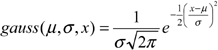
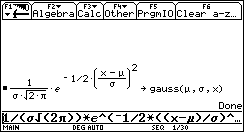
gauss describing the density function for normal distributions
In general there is a new chance for functions to be accepted by the students. Using CAS or programmable pocket calculators functions can be seen as an aid for evaluations complicated expressions. In traditional maths courses the students have to evaluate these long expressions by hand by themselves and they do not see the advantages of the use of functions. It is also a step to sturctured problem solving.
4. Experiences
The CAS is able to handle all the computing problems. It is not neccessary to find tricky ways for solving problems. Introducing new concepts we can start with very elementary and - due to that reason - very illustrative methods. For instance, we solved most problems of calculus using the limit of the quotient of differences. Therefore my students got a better understanding of the concept of a differential quotient and of derivatives. The problem of computing the limits was dedicated to the computer.
The possibility of recovering mathematical contents experimentally is very motivating for many students. The use of a computer gives many opportunities for experiments. However, experiments are quite time consuming and some students prefer traditional methods, because they are more convenient for them.
Using a CAS or the TI-92 we did not save time in the maths courses. There may be two reasons. First we spent much more time for introducing new mathematical concepts. The students tried to solve starting problems with elementary methods to obtain a better understanding for the new type of problems being treated. Secondly, we did not train special transformation rules for e.g. calculus. However it took a lot of time to learn the special techniques being required for an intensive use of the different windows on the TI-92 (home, graph, table, etc.).
The students defined many functions during three years. At the end of this time when the students have to apply all these functions to complex problems it was difficult for the students to remember the right name of the functions or to apply the functions to correct data types for the arguments.
References
[ Aspetsberger 1996]
Aspetsberger K.: Investigations on the Use of DERIVE for Students at
the Age of 17 and 18. The International DERIVE Journal, Vol. 3, No.
1, Research Information Ltd., Hemel Hempstead, England, 1996
[ Aspetsberger,
Fuchs 1996]
Aspetsberger K., Fuchs K.: DERIVE und der Rechner TI-92 im Mathematikunterricht
der 10. Schulstufe. International DERIVE and TI-92 Conference, Bonn
1996, p. 18-27.
[ Aspetsberger
1997]
Aspetsberger K.: Experiences about the use of the symbolic pocket calculator
TI-92 in math classes . The Third International Conference on Technology
in Mathematics Teaching ICTMT-3, Koblenz (CD-ROM).
[ Aspetsberger
1998a]
Aspetsberger K.: Teaching Integrals with the TI-92. A chance of making
a complex mathematical concept elementary. International Conference
on the Teaching of Mathematics, Samos, Greece, July 3-6, 1998, pp. 29-31.
[ Aspetsberger
1998b]
Aspetsberger K.: Probability Distributions in Math Courses with the
TI-92. Third International DERIVE/TI-92 Conference, Gettysburg, July
14-17, 1998.
[ Buchberger 1989]
Buchberger B.: Why Should Students Learn Integration Rules? RISC-
Linz Technical Report No. 89-7.0, Johannes Kepler University Linz, Austria.
[ Finney, Thomas,
Demana, Waits 1994]
Finney R.L., Thomas G.B., Demana F.D., Waits B.K.: Calculus: graphical,
numerical, algebraic. Addison-Wesley, 1994.
[ Heugl, Klinger,
Lechner 1996]
Heugl H., Klinger W., Lechner J.: Mathematikunterricht mit Computeralgebra-Systemen
(Ein didaktisches Lehrbuch mit Erfahrungen aus dem österreichischen
DERIVE-Projekt). Addison-Wesley, Bonn, 1996.
[ Heugl 1998]
Heugl H.: The Module Principle in Trigonometry. International Conference
on the Teaching of Mathematics, Samos, Greece, July 3-6, 1998, pp. 335-337.
[ Peschek 1998]
Peschek W.: Mathematical Concepts and New Technology. International
Conference on the Teaching of Mathematics, Samos, Greece, July 3-6, 1998,
pp. 242-244.
[ Schneider 1998]
Schneider E.: New Technology: a New Chance for "Old" Didactic Ideas?.
International Conference on the Teaching of Mathematics, Samos, Greece,
July 3-6, 1998, pp. 263-265.
[ Wurnig 1996]
Wurnig O.: Die Behandlung zweier anwendungsorientierter Aufgaben zur
Exponentialfunktion in Klasse 10 unter Verwendung von DERIVE. In:
Hischer & Weiß (Hgb.), Rechenfertigkeit und Begriffsbildung,
Verlag franzbecker, Hildesheim, 1996